Example of use
[1]:
import LMIPy
[2]:
LMIPy.__version__
[2]:
'0.4.0'
Collection objects: Searching
If you don’t know what data you are interested in advance, you can search by keywords and return a list of objects.
[15]:
c = LMIPy.Collection('tree cover', object_type=['layer','dataset'], app=['gfw'], limit=10)
[16]:
c
[16]:
Searching can be restricted with keyword arguments to specifically search types of items, applications, and more. If you want to render those items, you will need to do the following.
You can access items from a collection using subscripts, slices and more. Note that slicing, or selecting by element instantiates the Layer, Table, or Dataset object.
[17]:
c[0:3]
[17]:
[Dataset f3fc0f1e-aa26-49b6-8741-45df2eea9ac2 Brazil Land Cover,
 Dataset b3bfa285-ab43-4562-b2e0-0ab3e92c59e3 Brazil Land Cover 1985-2017,
 Layer 220080ec-1641-489c-96c4-4885ed618bf3 Brazil land cover - 2000-2016]
[18]:
c[-1]
[18]:
[19]:
l = c[-1]
l.map()
[19]:
Custom collections
As Collections are simply named groups of API entities (Layers, Datasets, or Widgets) you can create and manage your own given you have authrosation to do so.
Note that you can only view and manage your own custom Collections. See RW-API docs for more.
Creating a new Collection
Specify a list of valid objects, name, and application.
The resources list may be a list of LMIPy objects or a list of dicts specifying the type and id of each resource.
[8]:
layer_1 = LMIPy.Layer('0cba3c4f-2d3b-4fb1-8c93-c951dc1da84b')
layer_2 = LMIPy.Layer('d5b0a81b-70cd-4f33-860a-34a3c17867f3')
[9]:
# List of LMIPy objects
resource_list = [
    layer_1,
    layer_2
]
[12]:
c = LMIPy.Collection(
    attributes={
        'resources': resource_list,
        'name': 'Example Collection 1',
        'application': 'gfw'
}, token=<TOKEN>)
https://api.resourcewatch.org/v1/collection/5f5b5e7e055805001a08ee5c
[13]:
# Collection resources
c
[13]:
[15]:
# Collection attributes
c.attributes
[15]:
{'application': 'gfw',
 'name': 'Example Collection 1',
 'ownerId': '59db4eace9c1380001d6e4c3',
 'resources': [{'attributes': {},
   'id': '0cba3c4f-2d3b-4fb1-8c93-c951dc1da84b',
   'server': 'https://api.resourcewatch.org',
   'type': 'Layer'},
  {'attributes': {},
   'id': 'd5b0a81b-70cd-4f33-860a-34a3c17867f3',
   'server': 'https://api.resourcewatch.org',
   'type': 'Layer'}]}
Getting Collections by ID
Requires authorisation.
[ ]:
c = LMIPy.Collection(id_hash='5f5b5e7e055805001a08ee5c', token=<TOKEN>)
[24]:
c.attributes['name']
[24]:
'Example Collection 1'
[22]:
c
[22]:
Adding further resources
You may also add more resources to the Collection
[17]:
dataset_1 = LMIPy.Dataset('c92b6411-f0e5-4606-bbd9-138e40e50eb8')
[25]:
updated_c = c.add_resources(resources=[dataset_1], token=<TOKEN>)
Dataset c92b6411-f0e5-4606-bbd9-138e40e50eb8 added to Collection 5f5b5e7e055805001a08ee5c.
[26]:
updated_c.attributes['name']
[26]:
'Example Collection 1'
[27]:
updated_c
[27]:
Deleting custom collection
[4]:
c = LMIPy.Collection(id_hash='5f5b5e7e055805001a08ee5c', token=<TOKEN>)
[6]:
c.delete(token=<TOKEN)
Delete Collection Example Collection 1 with id=5f5b5e7e055805001a08ee5c?
> y/n
y
https://api.resourcewatch.org/collection/5f5b5e7e055805001a08ee5c
Deletion successful!
[8]:
try:
    c = LMIPy.Collection(id_hash='5f5b5e7e055805001a08ee5c', token=<TOKEN>)
except:
    print(f"Collection does not exist.")
Collection does not exist.
Dataset objects
Using known id’s you can instantiate a dataset object directly.
[3]:
ds = LMIPy.Dataset('044f4af8-be72-4999-b7dd-13434fc4a394')
ds
[3]:
You can access the attributes of a dataset.
[4]:
ds.attributes
[4]:
{'application': ['gfw', 'gfw-pro'],
 'attributesPath': None,
 'blockchain': {},
 'clonedHost': {},
 'connectorType': 'rest',
 'connectorUrl': None,
 'createdAt': '2019-09-19T15:25:32.570Z',
 'dataLastUpdated': None,
 'dataPath': None,
 'env': 'production',
 'errorMessage': '[Automatic Validation] ConnectorFailed -> Invalid Dataset',
 'geoInfo': False,
 'layerRelevantProps': [],
 'legend': {'binary': [],
  'boolean': [],
  'byte': [],
  'country': [],
  'date': [],
  'double': [],
  'float': [],
  'half_float': [],
  'integer': [],
  'keyword': [],
  'nested': [],
  'region': [],
  'scaled_float': [],
  'short': [],
  'text': []},
 'mainDateField': None,
 'name': 'Tree cover',
 'overwrite': False,
 'protected': True,
 'provider': 'gee',
 'published': True,
 'slug': 'Tree-cover',
 'sources': [],
 'status': 'saved',
 'subtitle': None,
 'tableName': 'UMD/hansen/global_forest_change_2013',
 'taskId': None,
 'type': None,
 'updatedAt': '2018-11-21T13:55:01.210Z',
 'userId': '596cde70824315350dd0f116',
 'verified': False,
 'widget': [],
 'widgetRelevantProps': []}
You can also access the metadata and vocabularies if they exist.
[5]:
ds.vocabulary[0].attributes
[5]:
{'application': 'gfw',
 'name': 'categoryTab',
 'resource': {'id': '044f4af8-be72-4999-b7dd-13434fc4a394', 'type': 'dataset'},
 'tags': ['landCover']}
[6]:
ds.metadata[0].attributes
[6]:
{'application': 'gfw',
 'createdAt': '2018-08-03T10:17:06.249Z',
 'dataset': '044f4af8-be72-4999-b7dd-13434fc4a394',
 'info': {'citation': '2000/2010, Hansen/UMD/Google/USGS/NASA',
  'color': '#a0c746',
  'description': 'Identifies areas of tree cover.',
  'isSelectorLayer': True,
  'name': 'Tree cover'},
 'language': 'en',
 'resource': {'id': '044f4af8-be72-4999-b7dd-13434fc4a394', 'type': 'dataset'},
 'status': 'published',
 'updatedAt': '2018-11-06T15:57:49.716Z'}
Queries on Datasets
Datasets can be queried via SQL, with a table returned. Currently this is only supported for Carto-type data:
[7]:
d = LMIPy.Dataset(id_hash='bd5d7924-611e-4302-9185-8054acb0b44b')
d
[7]:
[8]:
d.query('SELECT fid, ST_ASGEOJSON(the_geom_webmercator) FROM data LIMIT 5')
[8]:
| fid | st_asgeojson | |
|---|---|---|
| 0 | 0 | {"type":"MultiPolygon","coordinates":[[[[-6998... |
| 1 | 62 | {"type":"MultiPolygon","coordinates":[[[[-6927... |
| 2 | 343 | {"type":"MultiPolygon","coordinates":[[[[-6996... |
| 3 | 402 | {"type":"MultiPolygon","coordinates":[[[[-7004... |
| 4 | 682 | {"type":"MultiPolygon","coordinates":[[[[-6937... |
Layer Objects
Similarly, you can also instantiate a Layer object.
[9]:
ly = LMIPy.Layer(id_hash='dc6f6dd2-0718-4e41-81d2-109866bb9edd')
ly
[9]:
Layers can be visulized if appropriate via a call to Layer().map()
[10]:
ly.map()
[10]:
Tables
Tables are subclasses of Dataset objects. They are document datasets which can be instantiated and queried returning a dataframe object.
[11]:
t = LMIPy.Table(id_hash='86c7135a-855d-4f1b-9d67-f545a93281b3')
t
[11]:
[12]:
df = t.head(3)
df
[12]:
| City | Number_of_Days | _id | |
|---|---|---|---|
| 0 | Beijing | 14 | AWILuq8j8Jqrt1rp-STQ |
| 1 | San Francisco | 10 | AWILuq8j8Jqrt1rp-STT |
| 2 | Manama | 7 | AWILuq8j8Jqrt1rp-STU |
Queries to tables are returned in geopandas dataframe format.
[13]:
type(df)
[13]:
geopandas.geodataframe.GeoDataFrame
[14]:
t.query("SELECT * from data where City = 'San Francisco'")
[14]:
| City | Number_of_Days | _id | |
|---|---|---|---|
| 0 | San Francisco | 10 | AWILuq8j8Jqrt1rp-STT |
Create a Geometry object
Often you will need to perform some kind of intersect analysis between data held in datasets and tables and a geometry. We will now show you multiple ways to create your geometry objects.
From an ID
Vizzuality’s API holds geometry objects as a Geostore item. Geostore items are accessed by an id-hash. If you know the hash of your object already you can simply call a geometry like so:
[20]:
g = LMIPy.Geometry(id_hash='e8b6f974bcab5aefccd121654860be06')
g
[20]:
Geometry attributes
The attributes can be accessed as a dictionary.
[21]:
g.attributes
[21]:
{'areaHa': 16931274.241571266,
 'bbox': [-49.6113281249728,
  -9.77447583284213,
  -44.513671874972,
  -4.19348629349041],
 'geojson': {'crs': {},
  'features': [{'geometry': {'coordinates': [[[-47.8535156249717,
        -4.19348629349041],
       [-49.6113281249728, -9.77447583284213],
       [-44.513671874972, -9.25438811084709],
       [-47.8535156249717, -4.19348629349041]]],
     'type': 'Polygon'},
    'properties': None,
    'type': 'Feature'}],
  'type': 'FeatureCollection'},
 'hash': 'e8b6f974bcab5aefccd121654860be06',
 'info': {'use': {}},
 'lock': False,
 'provider': {}}
Geometry as a Table
Table method returns a dataframe of the geometry object. Map will add a Folium map with the geomerty rendered.
[22]:
g.table()
[22]:
| areaHa | bbox | geometry | id | use | |
|---|---|---|---|---|---|
| 0 | 1.693127e+07 | [-49.6113281249728, -9.77447583284213, -44.513... | POLYGON ((-47.8535156249717 -4.19348629349041,... | e8b6f974bcab5aefccd121654860be06 | {} |
Mapping the Geometry
Calling .map() will create a Folium map with the geomerty rendered.
[23]:
g.map()
[23]:
From Geojson - Points
You can create an object as you need on the fly from geojson. The act of creating an object will also register it to a Geostore service of your choice (locally, or on a remote server). You can create a geometry object from geojson Points and MultiPoints type data as follows:
[24]:
atts = {'geojson': {'type': 'FeatureCollection',
  'features': [{'type': 'Feature',
    'properties': {},
    'geometry': {'type': 'MultiPoint', 'coordinates': [[-4.29, 39.1097]]}}]}}

point = LMIPy.Geometry(attributes=atts, server='https://production-api.globalforestwatch.org')
point
[24]:
From Geojson - Polygons
You can create an object as you need on the fly from geojson. The act of creating an object will also register it to a Geostore service of your choice (locally, or on a remote server). You can create a geometry object from Geojson Polygon and Multipolygon type data as follows:
[25]:
atts={'geojson': {'type': 'FeatureCollection',
  'features': [{'type': 'Feature',
    'properties': {},
    'geometry': {'type': 'Polygon',
     'coordinates': [[[82.265625, 32.84267363195431],
       [77.34374999999999, 27.059125784374068],
       [85.4296875, 22.268764039073968],
       [90.3515625, 28.304380682962783],
       [87.5390625, 32.54681317351514],
       [82.265625, 32.84267363195431]]]}}]}}


g1 = LMIPy.Geometry(attributes=atts)
g1
[25]:
[26]:
g1.map()
[26]:
From a Shapely object
Shapely objects are at the root of popular python geolibraries such as Geopandas. We can recieve those geometry objects and create a Geometry object (simultaneously registering it in a Vizzuality Geostore server).
[27]:
import geopandas as gpd
[28]:
%%writefile ./sample.geojson
{"features":[{"properties":null,"type":"Feature","geometry":{"type":"Polygon","coordinates":[[[-43.1343734264374,-8.07358087603511],[-43.1327533721924,-8.08277985402466],[-43.1298887729645,-8.08181322762719],[-43.1103515625,-8.07815914647929],[-43.1094932556152,-8.07799981079283],[-43.1094932556152,-8.09641859926744],[-43.1103515625,-8.09645046495416],[-43.1187307834625,-8.0967372560211],[-43.1186878681183,-8.10273857778317],[-43.1186771392822,-8.10358831522616],[-43.1476235389709,-8.10358831522616],[-43.1477630138397,-8.10273857778317],[-43.1505310535431,-8.08645513764317],[-43.1517112255096,-8.08057041885644],[-43.1439757347107,-8.0795931648273],[-43.1448876857758,-8.07574785969913],[-43.1343734264374,-8.07358087603511]]]}}],"crs":{},"type":"FeatureCollection"}
Overwriting ./sample.geojson
[29]:
df = gpd.read_file('./sample.geojson')
df
[29]:
| geometry | |
|---|---|
| 0 | POLYGON ((-43.1343734264374 -8.073580876035111... |
[30]:
s = df.geometry[0]
print(f"Hello! 👋 I am a {type(s)}")
s
Hello! 👋 I am a <class 'shapely.geometry.polygon.Polygon'>
[30]:

[31]:
g = LMIPy.Geometry(s=s)
[32]:
g
[32]:
From Political Boundaries
We are able to return political boundaries (based on GADM data) using ISO, admin keys, down to admin-2 level. These should be passed in a dictionary to params. GADM 3.6 is currently used by default.
[33]:
params={
    'iso': 'BRA',
    'adm1': None,
    'adm2': None
}
admin = LMIPy.Geometry(parameters=params)
admin.map()
[33]:
From an admin geometry with an older GADM version
Alternatively, you can specify a different gadm version.
[34]:
params={
    'iso': 'BRA',
    'adm1': 1,
    'adm2': 1,
    'gadm': '2.7'
}
admin_v1 = LMIPy.Geometry(parameters=params)
admin_v1.map()
[34]:
From a Carto table and index
You can also return geometries directly from a Carto table (under the public WRI-01 account) using the table name and cartodb_id.
[35]:
params={
    'table': 'gfw_logging',
    'id': 123
}
row_geom = LMIPy.Geometry(parameters=params)
row_geom.map()
[35]:
Describe a Geometry
Return a title and textual description of a geometry in any language.
[36]:
g.map()
[36]:
[37]:
%%time
g.describe()
Title: Area in Microrregião de São Raimundo Nonato, Piauí, Brazil
Description: The regions habitat is comprised of Caatinga. This region has no Intact Forest. The area has a predominantly equatorial climate with dry winters. It is part of the Tropical and Subtropical Dry Broadleaf Forests biome. The location is predominantly land area. Area of 1.15kha located in a lowland area.
CPU times: user 26.1 ms, sys: 2.18 ms, total: 28.2 ms
Wall time: 1.49 s
[38]:
g.describe(lang='es') # same description but this time in Spanish
Title: Área en la Microrregião de São Raimundo Nonato, Piauí, Brasil
Description: El hábitat regiones se compone de Caatinga. Esta región no tiene bosque intacto. La zona tiene un clima predominantemente ecuatorial, con inviernos secos. Es parte del bioma secos tropicales y subtropicales de hoja ancha bosques. La ubicación es predominantemente la superficie terrestre. Área de 1.15kha situado en una zona de tierras bajas.
Second example of geodescriber, but considering a larger area.
[39]:
atts={'geojson': {'type': 'FeatureCollection',
  'features': [{'type': 'Feature',
    'properties': {},
    'geometry': {'type': 'Polygon',
     'coordinates': [[[82.265625, 32.84267363195431],
       [77.34374999999999, 27.059125784374068],
       [85.4296875, 22.268764039073968],
       [90.3515625, 28.304380682962783],
       [87.5390625, 32.54681317351514],
       [82.265625, 32.84267363195431]]]}}]}}


g2 = LMIPy.Geometry(attributes=atts)
g2
[39]:
[40]:
g2.map()
[40]:
[41]:
g2.describe()
Title: Area near Nepal, Asia
Description: The region is made up of different habitats, including Central Tibetan Plateau alpine steppe, and Upper Gangetic Plains moist deciduous forests. This region contains some Intact Forest. The most common environmental conditions of the area are polar tundra climate. The region is made up of several types of biomes, including Montane Grasslands and Shrublands, and Tropical and Subtropical Moist Broadleaf Forests. The location is predominantly land area. Area of 89.13Mha located in a mix of lowland and mountainous areas.
After running describe, the results are avaiable as geometry.description
[42]:
g2.description
[42]:
{'description': 'The region is made up of different habitats, including Central Tibetan Plateau alpine steppe, and Upper Gangetic Plains moist deciduous forests. This region contains some Intact Forest. The most common environmental conditions of the area are polar tundra climate. The region is made up of several types of biomes, including Montane Grasslands and Shrublands, and Tropical and Subtropical Moist Broadleaf Forests. The location is predominantly land area. Area of 89.13Mha located in a mix of lowland and mountainous areas.',
 'lang': 'en',
 'title': 'Area near Nepal, Asia'}
Add a satellite image to the map of your Geometry
Single images
The Geometry().map() method supports the return of recent satellite imagery. We calculate the centroid of your geometry and return the best, most recent image that intersects with that point. This is simply to provide context to your geometry. For point geometries we return the best cloud-free image we can find within a specified date range.
[43]:
# Create a point

atts = {'geojson': {'type': 'FeatureCollection',
  'features': [{'type': 'Feature',
    'properties': {},
    'geometry': {'type': 'MultiPoint', 'coordinates': [[-4.29, 39.1097]]}}]}}

point = LMIPy.Geometry(attributes=atts, server='https://production-api.globalforestwatch.org')
point
[43]:
[44]:
point.map(image=True, start='2018-01-01', end='2018-12-31')
[44]:
Composite images
Whereas for polygon-type geoms we return a cloud-free composite image clipped to your geometry.
[45]:
# Create a polygon

atts={'geojson': {'type': 'FeatureCollection',
  'features': [{'type': 'Feature',
    'properties': {},
    'geometry': {'type': 'Polygon',
     'coordinates': [[[-0.87890625, 43.329173667843904],
       [-1.6149902343749998, 42.75104599038353],
       [-1.1865234375, 42.35854391749705],
       [-0.6427001953125, 42.755079545072135],
       [-0.45043945312499994, 42.9524020856897],
       [-0.87890625, 43.329173667843904]]]}}]}}

g1 = LMIPy.Geometry(attributes=atts, server='https://production-api.globalforestwatch.org')
g1
[45]:
[46]:
g1.map(image=True, instrument='sentinel')
[46]:
Display a Layer and Geometry together
[47]:
atts={'geojson': {'type': 'FeatureCollection',
  'features': [{'type': 'Feature',
    'properties': {},
    'geometry': {'type': 'Polygon',
     'coordinates': [[[-48.131103515625, -0.6001172008725418],
       [-48.13934326171875, -0.9791088369866402],
       [-47.86331176757812, -0.9818550168696459],
       [-47.616119384765625, -0.8459165322899671],
       [-47.50213623046875, -0.7182123915862891],
       [-47.51861572265625, -0.5287095375108173],
       [-47.882537841796875, -0.5163504323777461],
       [-48.131103515625, -0.6001172008725418]]]}}]}}
g = LMIPy.Geometry(attributes=atts)
l = LMIPy.Layer(id_hash='3ef039ba-29c7-459d-aadd-66d6e6cc8f5e')
l
[47]:
[48]:
l.map(geometry=g)
[48]:
Intersecting Raster data with Geometry objects
Any Layer or Dataset objects based on an Earth Engine raster can be intersected with LMIPy.Geometry objects.
Dataset Intersections
In the first instance we show the result of an intersect between a geometry roughly bounding London, and a Population density layer.
[49]:
atts={'geojson': {'type': 'FeatureCollection',
  'features': [{'type': 'Feature',
    'properties': {},
    'geometry': {'type': 'Polygon',
     'coordinates': [
          [
            [
              -0.5712890625,
              51.28940590271679
            ],
            [
              0.48339843749999994,
              51.28940590271679
            ],
            [
              0.48339843749999994,
              51.781435604431195
            ],
            [
              -0.5712890625,
              51.781435604431195
            ],
            [
              -0.5712890625,
              51.28940590271679
            ]
          ]
        ]}}]}}

g = LMIPy.Geometry(attributes=atts)
[50]:
ds = LMIPy.Dataset(id_hash='a4e9c32d-d037-4c50-a893-967cad193537')
ds
[50]:
[51]:
ds.layers[0].map(geometry=g)
[51]:
Finally, you can call the intersect function on the dataset object to see a dictionary of values.
[52]:
ds.intersect(geometry=g)
[52]:
{'population-density': {'count': 138767,
  'max': 5984.53564453125,
  'mean': 1.5942131871343077,
  'min': 0.0,
  'stdev': 31.059972394495446,
  'sum': 221224.18133906648}}
Layer Intersections
Intersections against layers work in the same manner. Here we show an intersect between an area along Brazil’s coast and a Mangrove biomass density Layer.
[53]:
atts={'geojson': {'type': 'FeatureCollection',
  'features': [{'type': 'Feature',
    'properties': {},
    'geometry': {'type': 'Polygon',
     'coordinates':

[
          [
            [
              -52.16308593749999,
              -1.669685500986571
            ],
            [
              -46.9775390625,
              -1.669685500986571
            ],
            [
              -46.9775390625,
              0.7909904981540058
            ],
            [
              -52.16308593749999,
              0.7909904981540058
            ],
            [
              -52.16308593749999,
              -1.669685500986571
            ]
          ]
        ]
                 }}]}}

g = LMIPy.Geometry(attributes=atts)
[54]:
ly = LMIPy.Layer('3ef039ba-29c7-459d-aadd-66d6e6cc8f5e')
ly
[54]:
[55]:
ly.map(geometry=g)
[55]:
[56]:
ly.intersect(geometry=g)
[56]:
{'b1': {'count': 135511,
  'max': 32.262001037597656,
  'mean': 2.3417258825859957,
  'min': 0.5376999974250793,
  'stdev': 5.0781633479771395,
  'sum': 302242.0047789521}}
ImageCollection: Search for satellite images
You can search for Landsat-8 and Sentinel-2 imagery using the ImageCollection module as follows:
[57]:
ic = LMIPy.ImageCollection(lon=28.3, lat=-16.6, start='2018-08-01', end='2018-08-10') # n.b. lon/lat are temporarily flipped
[58]:
ic
[58]:
[59]:
type(ic)
[59]:
LMIPy.imageCollection.ImageCollection
All types of pythonic list mainipulation are supported on the image collection results. Including iteration:
[60]:
for i in ic[0:2]:
    print(i)
Image COPERNICUS/S2/20180808T075611_20180808T081515_T35KPB
Image LANDSAT/LC08/C01/T1_RT_TOA/LC08_172071_20180805
…and subsetting to access individual Images.
Images: Individual satellite tiles
[61]:
i = ic[0]
i
[61]:
[62]:
type(i)
[62]:
LMIPy.image.Image
You can access the Image attributes, which indicate the provinence of the tile.
[63]:
i.attributes
[63]:
{'provider': 'COPERNICUS/S2/20180808T075611_20180808T081515_T35KPB'}
Mapping Satellite Images
You can also display web-map tiles and the bounding-box of the satellite image.
[64]:
i.map()
[64]:
Classification of individual Satellite Images
[65]:
classified = i.classify()
classified
[65]:
[66]:
classified.map()
[66]:
Composite and classify satellite image collections
First grab a collection, specifying a point and time period.
[67]:
ic = LMIPy.ImageCollection(lon=28.271979, lat=-16.457814, start='2018-06-01', end='2018-06-20')
ic
[67]:
Next ask for a composite image based on your collection. By default it will be for Sentinel-2, but you may change this via an argument to Landsat.
[68]:
i = ic.composite()
i
[68]:
You can then map your composite image.
[69]:
i.map()
[69]:
You can take your composite image, and apply a land cover classifier based on our pre-trained models. These are Deepvel, and Segnet.
[72]:
c = i.classify(model_type='segnet', version='v2')
c
[72]:

[73]:
c.map()
[73]:
Construct Widgets
A demo of how to use LMIPy to construct widgets like those on our projects such as Global Forest Watch Dashboard pages.
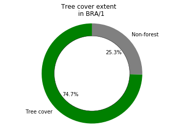
Tree cover example
[74]:
import matplotlib.pyplot as plt
%matplotlib inline
[75]:
# Get a datatable (Hansen)
table = LMIPy.Table('a20e9c0e-8d7d-422f-90f5-3b9bca355aaf')
table
[75]:
[76]:
iso = 'BRA'
administration = 1

sql = f"""
        SELECT
            SUM(area_extent) as value,
            SUM(area_admin) as total_area
        FROM data
        WHERE iso = '{iso}'
        AND adm1 = {administration}
        AND thresh = 30
        AND polyname = 'admin'
"""

results = table.query(sql=sql)
results
[76]:
| total_area | value | |
|---|---|---|
| 0 | 1.527330e+07 | 1.140593e+07 |
[77]:
sizes = [results.value[0], results.total_area[0] - results.value[0]]
colors = ['green','grey']
labels = ['Tree cover', 'Non-forest']

fig1, ax1 = plt.subplots()
ax1.pie(sizes, labels=labels, autopct='%1.1f%%',
        shadow=False, startangle=90, colors=colors)
ax1.axis('equal')
centre_circle = plt.Circle((0,0),0.75,color='black', fc='white',linewidth=0.5)
fig1 = plt.gcf()
fig1.gca().add_artist(centre_circle)
plt.suptitle('Tree cover extent')
plt.title(f'in {iso}/{administration}')
plt.show()
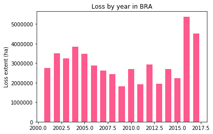
Tree cover loss example
[78]:
sql = """
SELECT
    polyname, year_data.year as year,
    SUM(year_data.area_loss) as area

FROM data
WHERE polyname = 'admin'
AND thresh= 30
GROUP BY polyname, iso, nested(year_data.year)
"""
global_loss = table.query(sql=sql)
global_loss.head()
[78]:
| area | iso | polyname | year | |
|---|---|---|---|---|
| 0 | 2.746361e+06 | BRA | admin | 2001 |
| 1 | 3.507049e+06 | BRA | admin | 2002 |
| 2 | 3.248527e+06 | BRA | admin | 2003 |
| 3 | 3.848771e+06 | BRA | admin | 2004 |
| 4 | 3.486563e+06 | BRA | admin | 2005 |
[79]:
iso='BRA'
loss_data = list(global_loss[global_loss['iso'] == f'{iso}']['area'])
years = list(global_loss[global_loss['iso'] == f'{iso}']['year'])

width = 0.66
fig, ax = plt.subplots()
rects1 = ax.bar(years, loss_data, width, color='#FE5A8D')

# add some text for labels, title and axes ticks
ax.set_ylabel('Loss extent (ha)')
ax.set_title(f'Loss by year in {iso}')
plt.show()
Creating a local backup of Data objects
Save a local backup of a collection to a specified path. This creates a folder containing a JSON for each dataset and it’s associated Layers, Metadata and Vocabularies.
[80]:
col = LMIPy.Collection(app=['gfw'], env='production')
[81]:
path = './LMI-BACKUP'
[82]:
col.save(path)
0%| | 0/330 [00:00<?, ?it/s]
Saving to path: ./LMI-BACKUP
100%|██████████| 330/330 [01:29<00:00, 3.67it/s]
Save complete!
Load Data objects from local backup
You can also load a previous version from local backup.
[84]:
import os
[85]:
files = os.listdir(path)[0:3]
files
[85]:
['a92ceeea-684a-4d39-89e1-4ca97673cb5a.json',
 'b70f070b-c9ae-4452-aa8e-2280a2604666.json',
 '89755b9f-df05-4e22-a9bc-05217c8eafc8.json']
[86]:
ds_id = files[0].split('.json')[0]
ds_id
[86]:
'a92ceeea-684a-4d39-89e1-4ca97673cb5a'
[87]:
dataset = LMIPy.Dataset(ds_id)
[88]:
dataset
[88]:
[89]:
backup = dataset.load(path)
[90]:
backup
[90]:
[ ]: